Kinetic Monte Carlo
KMC bridges the gap between regular Monte Carlo sampling procedures and real time dynamics. It is useful for systems in which multiple events are occurring, such as MBE or CVD growth. The transition probabilities are directly tied to physical rates, establishing a “dynamical hierarchy” of events. In the dynamical hierarchy, events with lower energy barriers have a high probability of occurring sooner than events with high energy barriers. Therefore, events that occur at a low physical rate are rare.
In our simulation of film growth, we can treat deposition and hopping as two independent events, which occur at different rates governed by relative energy barriers. The rate of deposition, \(R_{d},\) is specified by the atomic flux. For MBE, this is typically one monolayer per second. The rate of diffusion of a surface atom, i is
\[r_{i}=\omega e^{(\Delta E_{i}/k_{B}T)}\label{eq:1}\]
where \(\omega\) is the attempt rate, \(k_{b}\) is the Boltzmann constant, T is temperature, and \(\Delta E_{i}\) is the energy barrier for atom i to leave its current position and settle in a new one. Note that when \(\Delta E_{i}\) is zero, \(r_{i}=\omega.\) The total rate for all possible processes is then
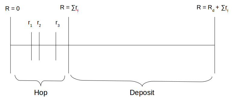
\[R_{total}=R_{d}+\sum_{i=1}^{N}r_{i}\label{eq:2}\]
for a system of N atoms. By this approach, a deposition event will occur with probability \(P_{d}=\frac{R_{d}}{R_{total}}\), and atom i will hop with probability \(P_{i}=\frac{r_{i}}{R_{total}}\).
There are a variety of methods for choosing an event based on this information. The n-fold-way involves selecting a quasi-random number between 0 and \(R_{total}\) with uniform probability. As shown in Figure 1, the position of this random number along the continuum determines if a new atom is deposited or if an existing atom hops. It also determines which existing atom hops. The chosen event is then executed, and the rates updated to reflect the new state. This effectively avoids the waste of computation time associated with many failed attempts to move a specific atom.
(Approximate) Off-Lattice Monte Carlo
The nature of heteroepitaxy disallows the assumption that an adatom will occupy a periodic lattice position. When materials have different equilibrium bond lengths and bond energies, there is a very real possibility that it will be more energetically favorable for an adatom to occupy some position along a continuum between lattice sites. This significantly complicates growth simulations, however, because the space must be described as a potential energy landscape ridden with local minima, rather than a discrete set of potential moves.
In an on-lattice algorithm, rates could be calculated for every potential move and stored in a rate catalog to be accessed later. One has to be more clever for off-lattice situations. In this case, atoms sit at local minimum energy positions, and they must overcome a potential energy barrier, \(\Delta U,\) in order to move. Then the hopping rate from site i to site j will be:
\[r_{ij}=\omega e^{(-\Delta U_{ij}/k_{b}T)}\label{eq:3}\]
The formal way to calculate \(\Delta U_{ij}\) would be to find the difference between the local energy minimum and its neighboring saddle point where \(\nabla U=0.\) Since these values are determined by all of the atoms in the configuration space, the act of finding and calculating them is rather computationally expensive. Instead, we will make an approximation based on the potential energy difference between the adatom in its current configuration, and the potential energy of the relaxed void as if the adatom had been removed.
Empirical Potential
The potential energies of different configurations will be calculated using the empirical Lennard-Jones potential. For an atom i interacting with another atom, j:
\[U_{ij}=\varepsilon_{ij}[(\frac{r_{m}}{r_{ij}})^{12}-2(\frac{r_{m}}{r_{ij}})^{6}]\]
where \(\varepsilon_{ij}\) is the potential well minimum, which occurs at \(r_{m}\), and \(r_{ij}\) is the measured distance between the two atoms. In physical terms, \(\varepsilon\) is the chemical bond energy and \(r_{m}\) is the nearest neighbor distance in a crystal. The force on an atom in an unstrained lattice is zero at \(r_{m}.\) In a heteroepitaxial film, the binding energy and nearest neighbor distance between two adatoms will be different than for two substrate atoms. The interaction of an adatom, \(a\), with a substrate atom, s, will be described by some average in bond character. Explicitly, \(r_{m,a-s}=\frac{1}{2}(r_{m,a}+r_{m,s})\) and \(\varepsilon_{a-s}=\sqrt{\varepsilon_{a}\varepsilon_{s}}.\)
Relaxation: Nonlinear Conjugate Gradient
When an atom hops or is deposited, it will initially arrive in a nonequilibrium position. It (and all of its neighbors) must then move towards the lowest energy configuration. The direction that they move depends on the gradient of the potential energy landscape. In particular, the force on each atom points in the direction of lowering its potential energy at the fastest rate. It does not necessarily point towards minimum energy position, however.
A relatively fast way to find the minimum energy position is the conjugate gradient method. The force on each atom, \(\Delta x_0\), is initially calculated. The minimum energy along this direction is determined using a line search. The energy is sampled at various points, \(x_1 = x_0 + \alpha \Delta x_0\), along the direction of this vector and each atom is moved to the position with a value of \(\alpha\) that minimizes the energy of the system. The direction of the force at this new position is calculated and the process is repeated. If the energy of the system is a linear system of equations that is symmetric and positive-definite, then this algorithm is guaranteed to eventually find a local minimum energy configuration.
The conjugate gradient method can be extended to nonlinear systems with the addition of another term when calculating the direction of the minimum energy line search. Rather than moving along the direction of the force vector, a direction
\[s_n = \Delta x_n + \beta_n s_{n-1}\]
is chosen where \(\beta_n\) is the conjugate step size. The initial value \(s_0\) is chosen as \(\Delta x_0\). Several forms for \(\beta\) exist in the literature; the Polak-Ribière formalism was used here:
\[\beta_n = \frac{\Delta x_n^\intercal (\Delta x_n - \Delta x_{n-1})}{\Delta x_{n-1}^\intercal \Delta x_{n-1}}\]
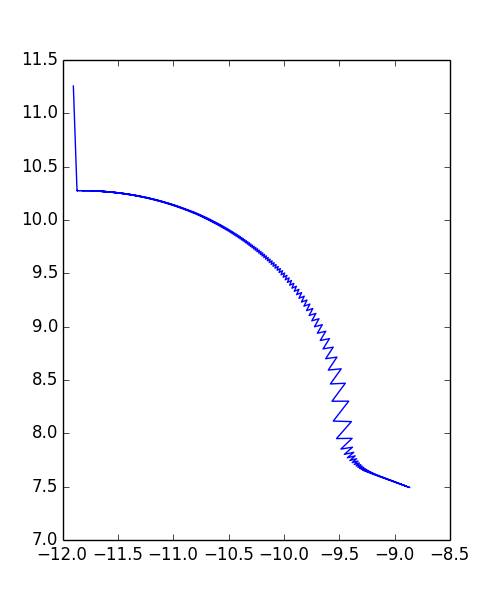
The line search is then performed for positions \(x_{n+1} = x_n + \alpha s_n\) and this process is repeated until the minimum energy is found. Figure 2 shows an example path of an atom searching for the minimum energy position using this method.
In practice, the minimum energy is defined as a configuration where the forces on each particle are so small that they can be neglected. This cutoff point was chosen as \(10^{-2}\) eV / \(\buildrel _\circ \over {\mathrm{A}}\).